When is a Gaussian prior “the same kind of thing”?

Learning notes · Raj Mahat · Georgia Tech

Computational notes on the Feldman–Hájek theorem and what it means for building priors for groundwater heads: which nonstationary features (wells, leakage, a conductivity lens) can be added as a correction to a stationary SPDE prior, and which force the operator itself to change.

Two Gaussian measures are equivalent iff a single, infinitely resolved sample cannot tell them apart. If one perfect sample can, they are mutually singular.

Read the notes (PDF) Chapter 1 notebook Source on GitHub

Chapter 1 · Feldman–Hájek and measure equivalence

Step	What the computation shows
Finite dimensions	Non-degenerate Gaussians are always equivalent; singularity needs a degenerate support.
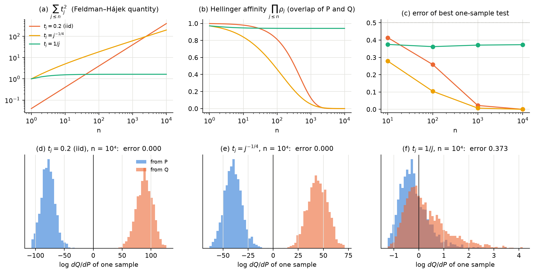
Infinitely many coordinates	A 20% variance change in every coordinate becomes perfectly detectable from one sample; equivalence holds iff Σ t_j² < ∞ (Kakutani).
Mean shifts	Equivalent iff the shift lies in the Cameron–Martin space; for the SPDE prior that is H², so a point well is singular.
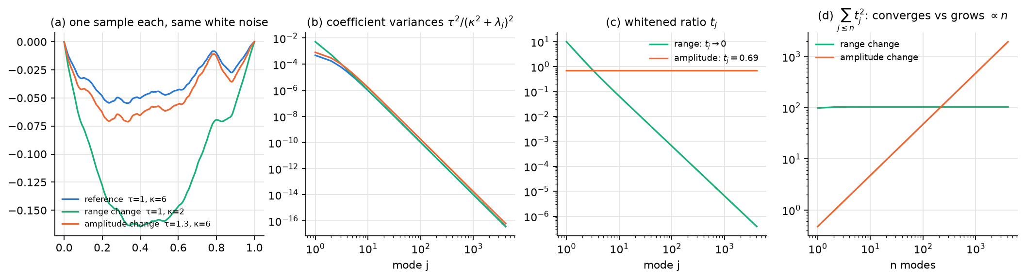
Range vs amplitude	Changing the range κ looks dramatic but is equivalent; changing the amplitude τ looks mild but is singular. One sample pins τ, never κ.
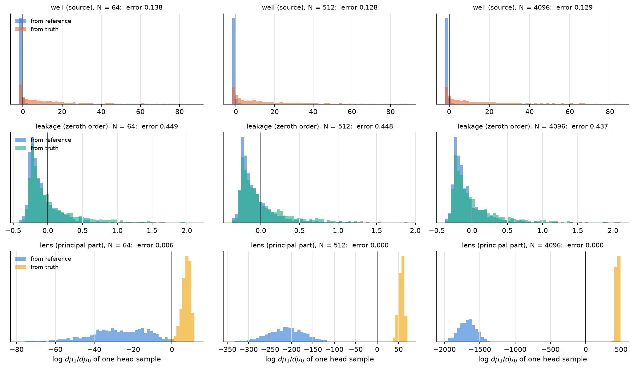
1D leaky aquifer	Well and leakage: ‖T‖ flat under refinement. Conductivity lens: ‖T‖ ∝ √N, and one head field identifies it.

Feldman–Hájek sum, Hellinger affinity and one-sample test error for three perturbation sequences — Only the perturbation that decays fast enough (t_j = 1/j) keeps a permanent overlap between P and Q.

Samples and spectra for range and amplitude changes — The range change (green) looks most different yet is equivalent; the amplitude change (orange) is singular because it persists at every fine scale.

One-sample likelihood-ratio histograms for well, leakage and lens — One head field: test error is stable under refinement for the well and leakage (equivalent) and drops to zero for the lens (singular).

Coming next

Whitening and the operator T in 2D; why a conductivity lens acts as multiplication by K⁻² − 1; how a finite-rank model sees T through sample covariances (Marchenko–Pastur, BBP); centred vs non-centred MCMC.