Differentiable plasticity FEM in JAX

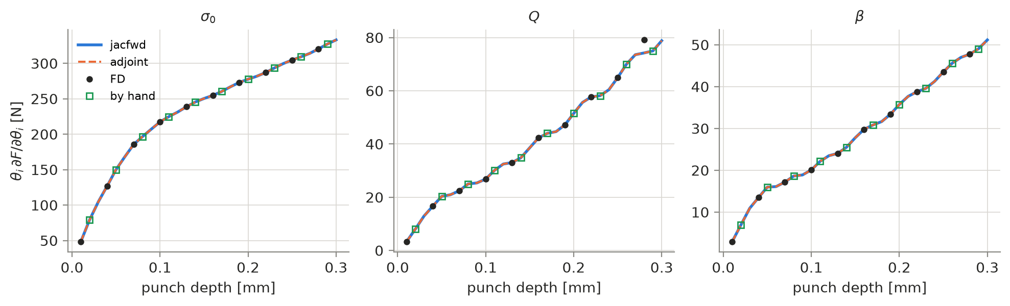
A mechanical test never measures the hardening law. It measures the law after it has passed through the local plastic response, equilibrium with contact, the loading history and the readout. These notes build a small, fully differentiable punch-test model in JAX and follow, step by step, how information about the law travels to the measured load, and how its derivatives are computed exactly.

1 · J₂ plasticity with combined hardening

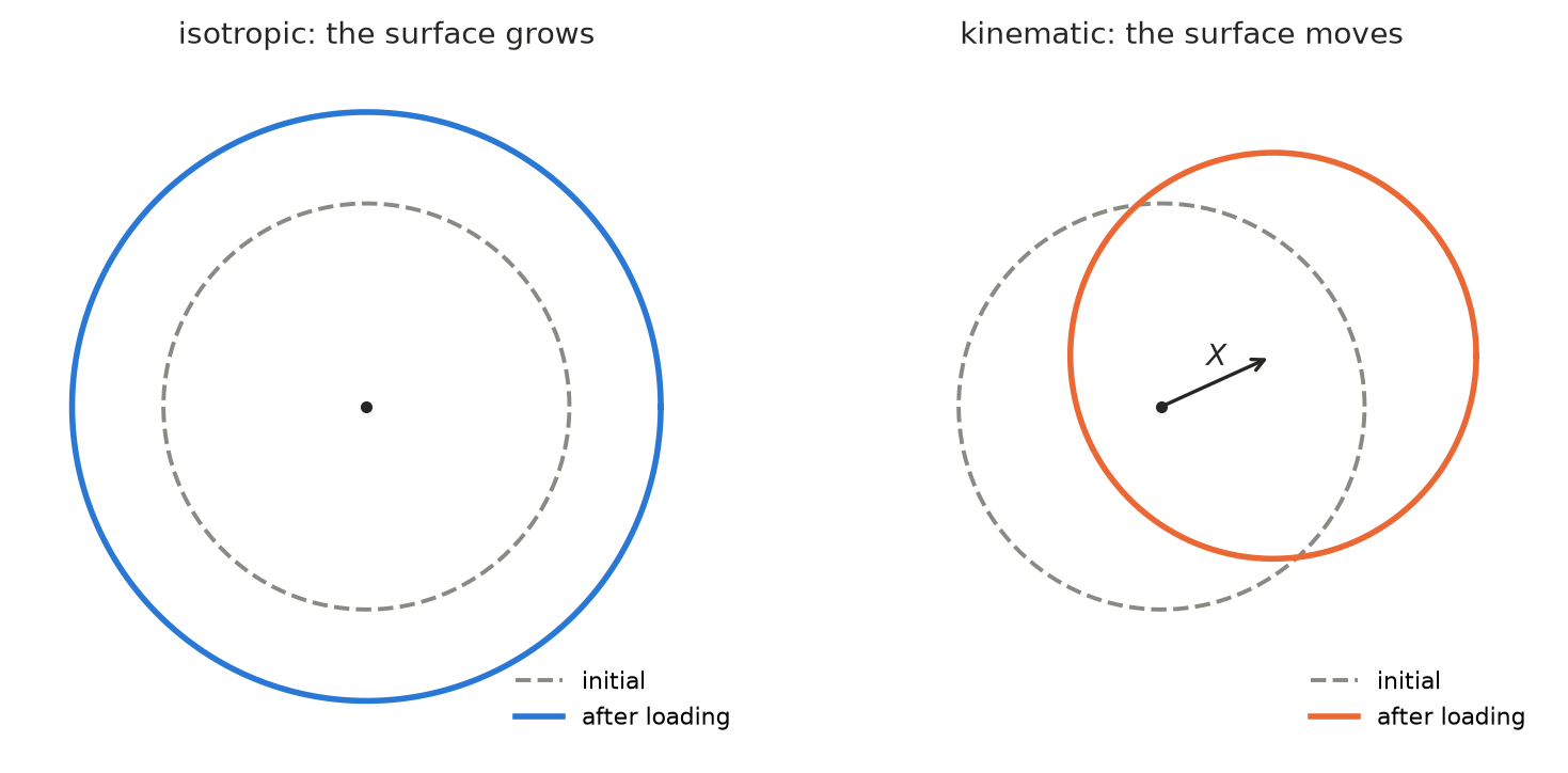
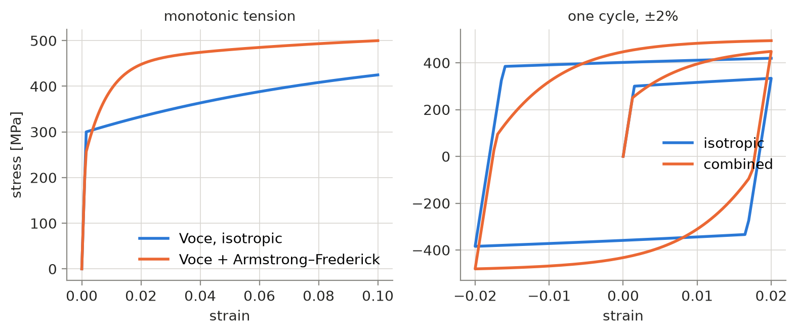
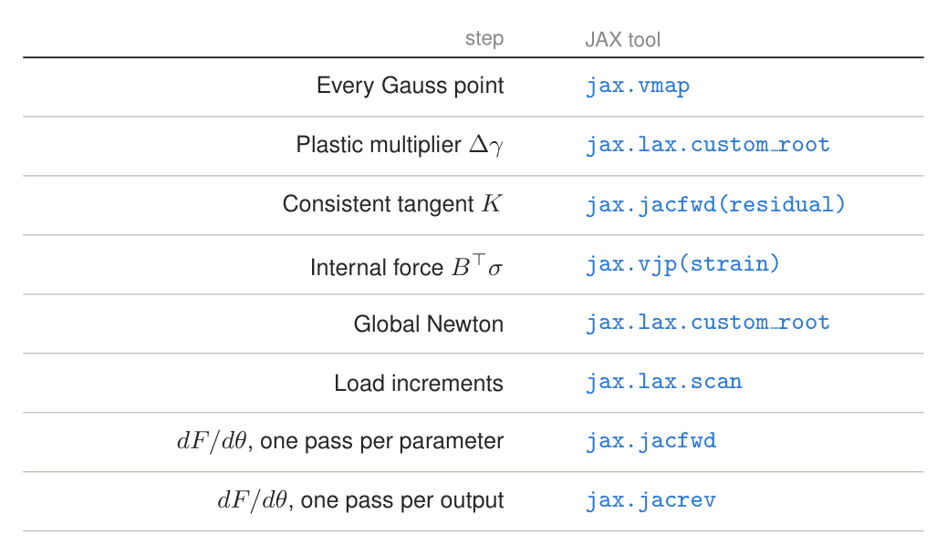
Voce isotropic hardening grows the elastic domain; Armstrong–Frederick kinematic hardening moves it. The backward-Euler return map reduces to one scalar equation for the plastic multiplier, solved inside jax.lax.custom_root, so the consistent tangent is a single jax.jacfwd. It matches the textbook closed form to round-off.

2 · The forward solve: one load increment at a time

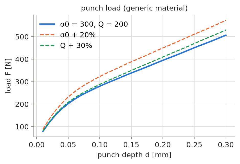
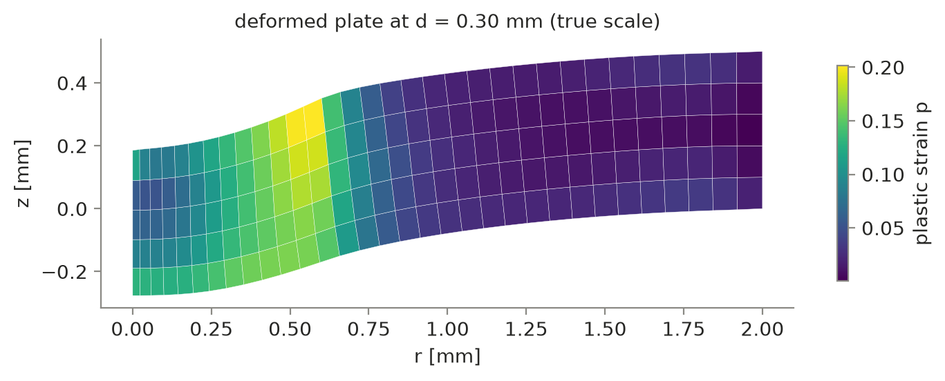
The punch is pushed into the plate in small steps of depth \(d_1, d_2, \dots, d_N\). Each step (an increment \(k\)) is a full nonlinear solve: find the nodal displacements for which the plate is in equilibrium, every Gauss point satisfies the plasticity law, and the plate does not pass through the punch. Once that is found, the plastic state is stored (committed) and becomes the starting point for the next step. The punch load \(L_k\) is read off at the end of each step, which gives the load–depth curve.

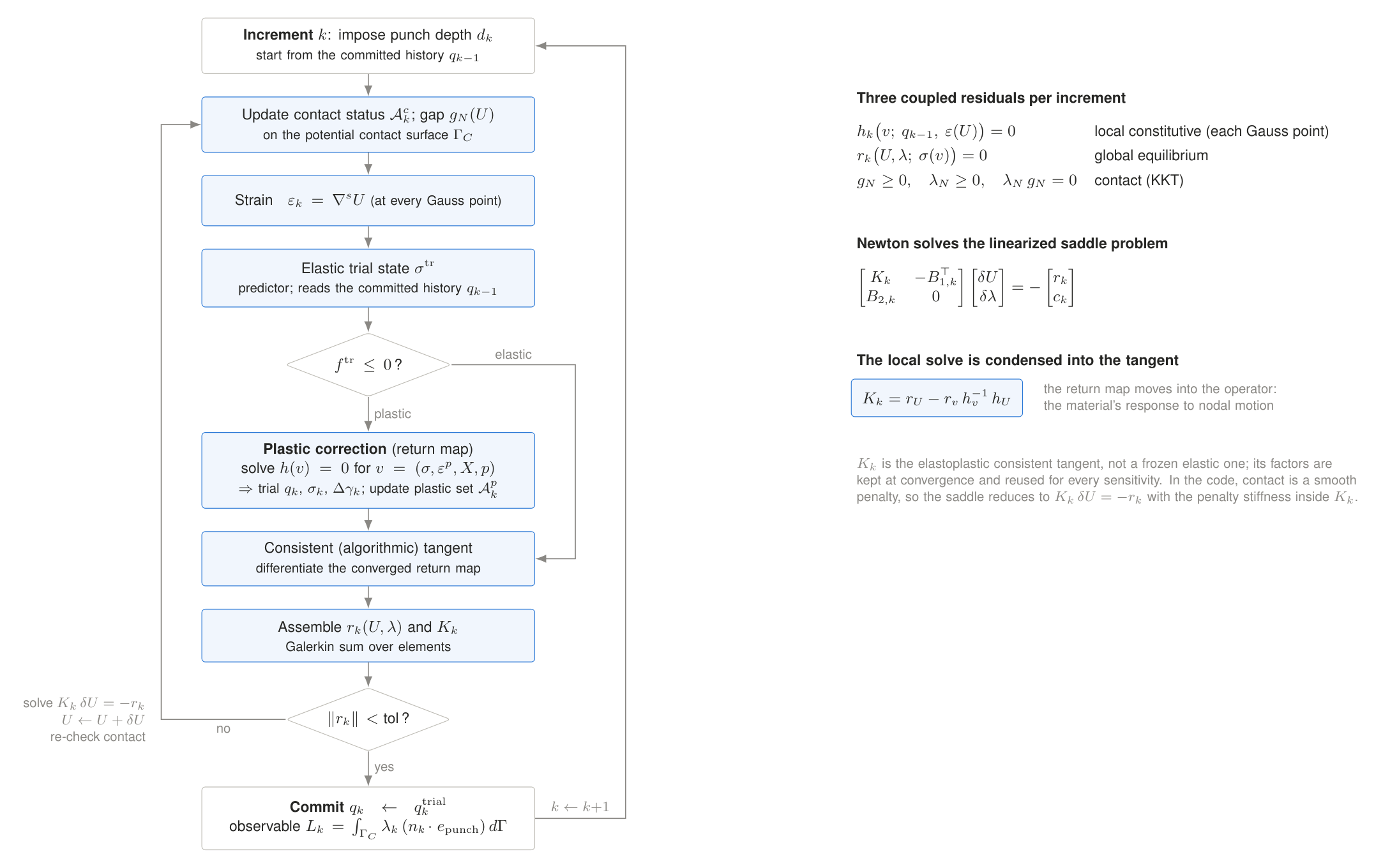
Reading the flowchart (left, top to bottom). Impose the new depth \(d_k\), starting from the stored history \(q_{k-1}\). Check which nodes touch the ball. Compute the strain at every Gauss point from the current displacements. Assume the step is elastic (the trial stress); if the trial stress lies inside the yield surface (\(f^{\rm tr}\le 0\)) it is accepted, otherwise the return map pulls it back onto the surface and updates the plastic variables. Differentiate that converged local update to get the consistent tangent, assemble the global residual \(r_k\) and stiffness \(K_k\), and take a Newton step. Repeat until the residual is small, then commit the history and read the load.

The right side says the same thing in equations. Three sets of conditions must hold together: the material law at every Gauss point (\(h_k=0\)), force balance (\(r_k=0\)), and contact (gap \(g_N\ge0\), pressure \(\lambda_N\ge0\), and pressure only where the gap is closed). Newton linearizes all of them at once. The key step is the boxed formula: the local unknowns can be eliminated, so the material's whole response is folded into one matrix, \(K_k = r_U - r_v h_v^{-1} h_U\) ("how the nodes push back when moved, after the material has re-equilibrated"). That factorized \(K_k\) is reused, unchanged, for every derivative in Section 3.

Six building blocks

Everything in Section 3 is assembled from six small maps. Each panel below shows one of them as a pipeline: the input on the left, the output on the right, and the formula underneath.

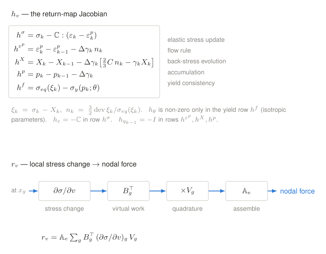
\(h_v\), the local block. The five equations a Gauss point must satisfy in one step: stress from elastic strain, the flow rule, back-stress evolution, accumulation of plastic strain, and staying on the yield surface. Its Jacobian \(h_v\) is what the return map inverts. Note where things enter: the parameters \(\theta\) appear only in the last (yield) row, through \(\sigma_y(p;\theta)\); the strain enters only the stress row; the stored history enters only the three evolution rows. \(r_v\), local to global. A change in stress at a Gauss point becomes a nodal force by the usual finite-element route: multiply by \(B^\top\) (virtual work), weight by the Gauss volume, and add up over elements.

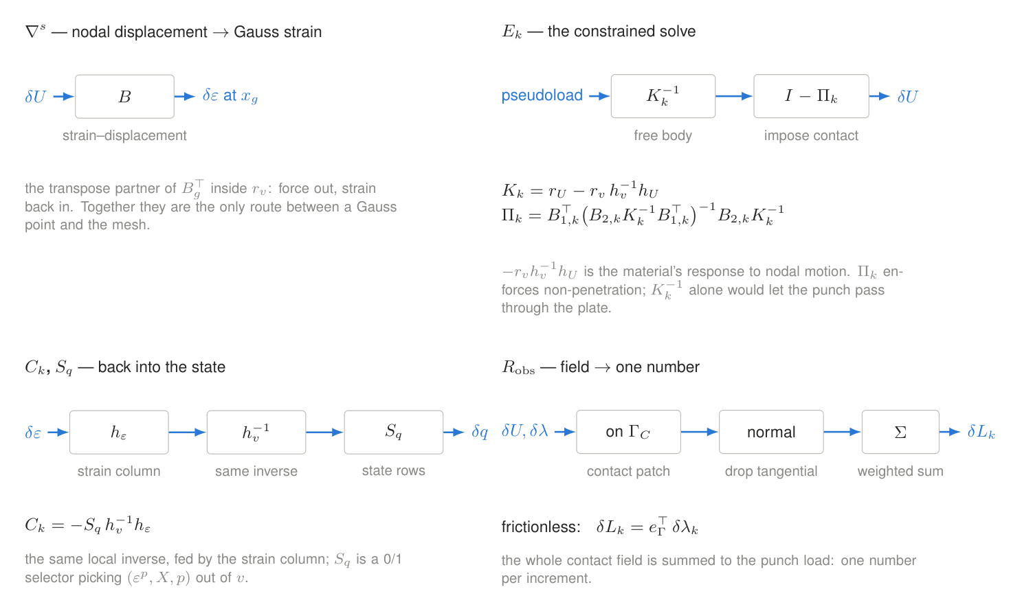
\(\nabla^s\) (top left) is the opposite direction: nodal displacement to strain at each Gauss point, through \(B\). \(E_k\) (top right) answers "given extra forces, how do the nodes move?": solve with the tangent \(K_k\), then project with \(\Pi_k\) so the plate still respects contact (without it the punch could pass through the plate). \(C_k,\ S_q\) (bottom left) turn a strain change back into a change of the stored history, using the same local inverse \(h_v^{-1}\); \(S_q\) just picks the history entries out of \(v\). Readout (bottom right): of all the fields, only the contact pressure on the contact patch is measured; summing its normal part gives the single number \(\delta L_k\).

3 · How a parameter change travels to the load

The question of this section: if \(\sigma_0\), \(Q\) or \(\beta\) is nudged by \(\delta\theta\), how much does the load at each depth change? The answer is the Jacobian \(J=\partial L/\partial\theta\) (one row per depth, one column per parameter). The charts show that computing it needs no new solver, only the building blocks above, reused in a fixed order.

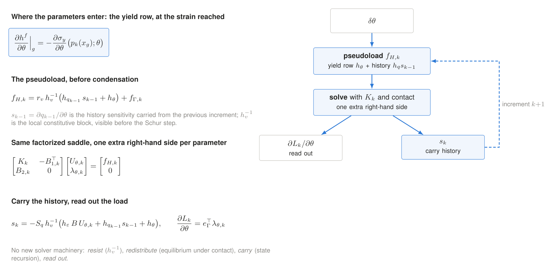
Four moves per increment (follow the blue boxes on the right).

1. Source. The parameters touch only the yield row (top-left box): a nudge to \(\theta\) shifts the yield stress at the plastic strain each Gauss point has reached. Elastic points feel nothing.
2. Pseudoload. That shift, plus whatever the earlier increments already changed in the history (\(s_{k-1}=\partial q_{k-1}/\partial\theta\)), is pushed through \(h_v^{-1}\) (the material resists) and \(r_v\) to become an equivalent set of nodal forces \(f_{H,k}\). The extra term \(f_{\Gamma,k}\) is the corresponding contribution from the contact rows.
3. Solve. Those forces are applied to the same factorized system as the forward Newton step: one extra right-hand side per parameter. This gives how the displacements and contact pressures move, \(U_{\theta,k}\) and \(\lambda_{\theta,k}\).
4. Carry and read out. Two things are kept: the new history sensitivity \(s_k\), which feeds the next increment (dashed loop), and the load sensitivity \(\partial L_k/\partial\theta\), read off the contact pressure.

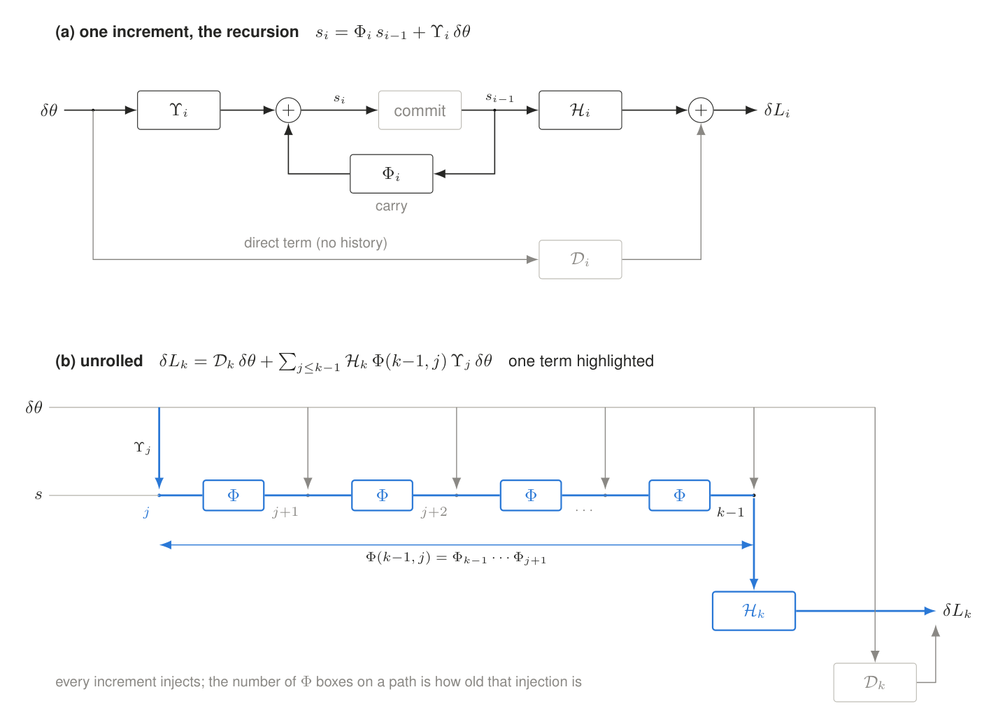
The same thing as a signal-flow diagram. (a) Per increment, the bookkeeping is linear: the new history sensitivity is the old one carried forward, plus what this increment injects, \(s_i=\Phi_i s_{i-1}+\Upsilon_i\,\delta\theta\). The load change is read from the history (\(\mathcal H_i\)) plus a direct part that needs no history (\(\mathcal D_i\)). Here \(\Upsilon\) = "inject", \(\Phi\) = "carry", \(\mathcal H\) = "read through the history", \(\mathcal D\) = "read directly". (b) Unrolling over increments: every increment injects something, and an injection made at step \(j\) reaches the load at step \(k\) only after being carried through \(k-1-j\) \(\Phi\) boxes (one path highlighted in blue). So the load at depth \(k\) is the sum of contributions of every earlier step, each weighted by how far it has been carried.

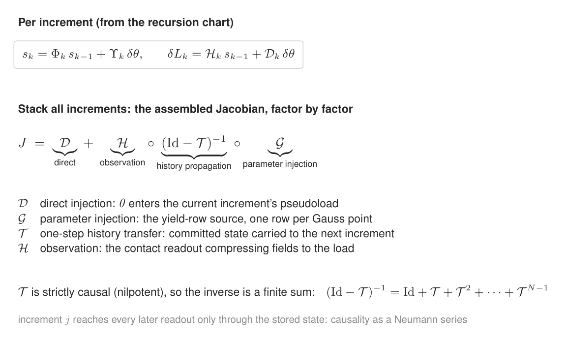
Stacking all increments turns those per-step boxes into four operators, and the full Jacobian factors as: inject (\(\mathcal G\)), propagate through history (\((\mathrm{Id}-\mathcal T)^{-1}\)), observe (\(\mathcal H\)), plus the direct part (\(\mathcal D\)). Because a step can only affect later steps, \(\mathcal T\) shifts information strictly forward in time, so the inverse is an exact finite sum: this is the unrolled picture above, written as one formula.

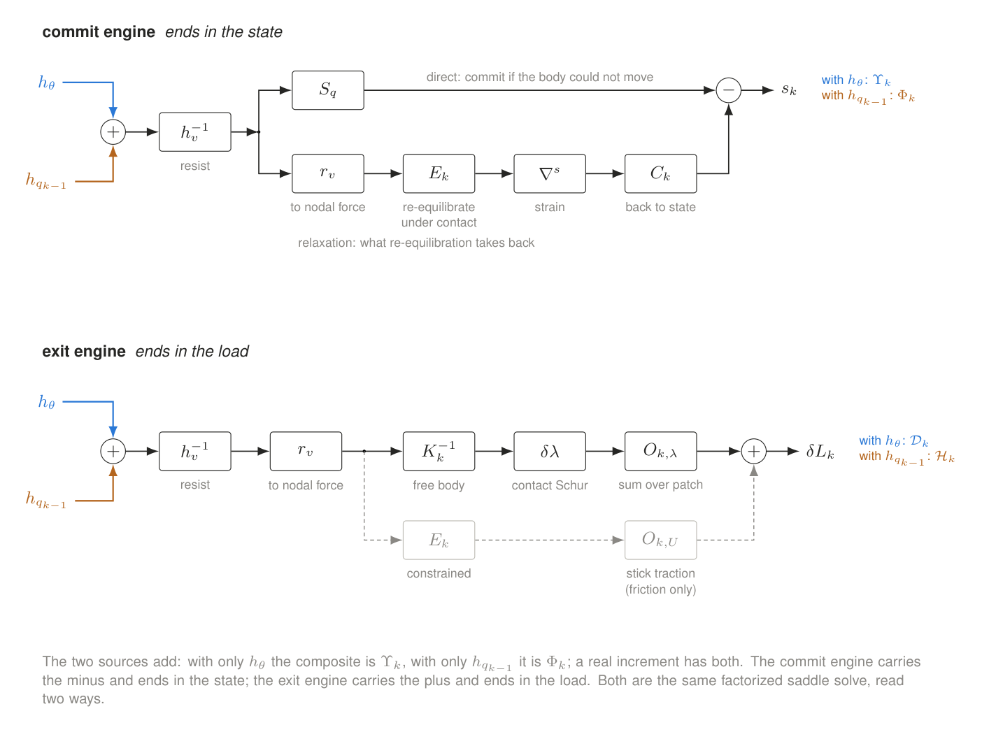
What is inside \(\Upsilon,\Phi,\mathcal H,\mathcal D\). All four are the same chain of building blocks, fed by one of two sources: the parameter source \(h_\theta\) (blue) or the history source \(h_{q_{k-1}}\) (orange). The commit path (top) ends in the stored state: the local block resists the change, and what the rest of the plate gives back after re-equilibrating (\(r_v\to E_k\to\nabla^s\to C_k\)) is subtracted. Fed by \(h_\theta\) it is \(\Upsilon_k\), fed by the history it is \(\Phi_k\). The exit path (bottom) ends in the load instead, through the contact pressure; fed by \(h_\theta\) it is \(\mathcal D_k\), fed by the history it is \(\mathcal H_k\). The grey dashed branch only matters with friction and is zero in this frictionless model.

4 · A local Bayesian view with three parameters

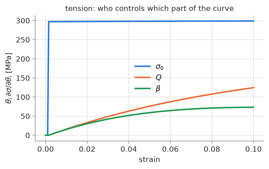
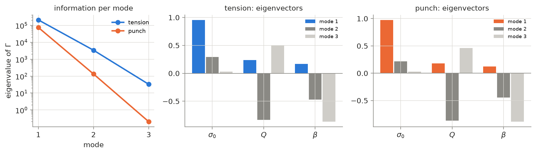
Around one anchor, the data add precision Γ = J^TΣ⁻¹J. Its eigenvectors are the combinations of (σ₀, Q, β) that a test pins down or leaves loose; along mode i the posterior variance shrinks by 1/(1+λ_i).

Where this leads

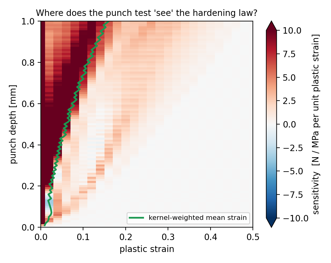
The same machinery can ask where in plastic-strain space, at each depth, the punch load is sensitive to the hardening law at all. A first look, work in progress:

Generic material and geometry, small-strain teaching model built on core JAX. This page shares the write-up and figures only.

Click any figure to open it at full size.